

Visualizing CTX DTMs in 3D Using QGIS
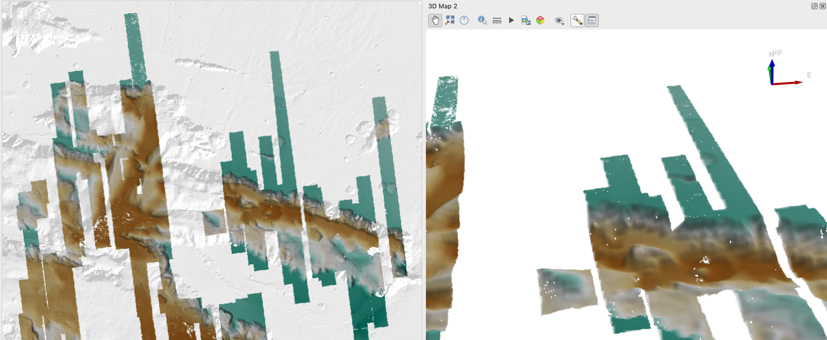
The results of this tutorial, a 3D visualization in Valles Marineris composed of 83 Mars Reconnaissance Orbiter (MRO) Context Camera (CTX) Digital Terrain Models (DTMs).
This is an in progress draft example. Please feel free to test, but use with caution!
In this tutorial, you will learn how to:
- searching for CTX DTMs using the STAC API
- creating a GDAL Virtual Format or VRT of a merge of the discovered DTMs
- use the QGIS hillshade tool to create a beautiful hillshade of the merged DTMs
- create a 3d interactive visualization using the QGIS 3d map capabilities
This tutorial is linking together a number of other tutorials (linked above), so if you have any issues, check those out or add a question in the comments section at the end. If you have changes you would like to see, consider submitting them back to the community via a pull request by clicking the “Edit page” link in the top right of this page.
This tutorial requires that you have the following tools installed on your computer:
| Software Library or Application | Version Used |
|---|---|
| QGIS | 3.30.1 |
| pystac-client | 0.6.1 |
| GDAL | 3.6.3 |
For this tutorial, a region of interest (ROI) around Valles Marineris was selected. This is because quite a few DTMs are in that area and the vertical relief is high. The pystac-client library and a simple python script were used to find the 83 DTMs in the ROI.
|
|
Line by line, this code:
- Imports the
pystac_clientlibrary for use. - Creates a
Clientobject that is the connection to the search API. - Performs a search on the API in the collection named
mro_ctx_controlled_usgs_dtmsand for all data that intersect the bounding box (bbox). No limit on the number of returned items is provided.* search.items()returns a list of STAC Items . The full line of code uses a list comprehension to extract the URL of the DTM from the downloadable assets associated with each Item. The end result is a list of URLs to DTMs stored in an S3 bucket.
Next, the discovered DTMs will be merged together into a single file. One could download each DTM locally and then merge them. Because these data are cloud optimized and well suited for streaming, it is more efficient to simply make a virtual file or VRT that points at the source data. The following python snippet creates a VRT.
|
|
Line by line, this code:
- Imports the
gdallibrary for use. - Prepends every URL in the previously created URL list with
/vsicurl. The vsicurl prefix to files tells GDAL to use a remote file accessor to read the files. This prefix allows streaming of the data from a network accessible source to a local computer for visualization and analysis. - Build a local, on-disk VRT that be loaded into QGIS and visualized.
- Flush the GDAL I/O cache, forcing the VRT to write to disk.
By combining these together, a script can be created to generate a VRT for any ROI. Create a file named find_dtms_and_make_vrt.py. Paste the code below into the file.
|
|
Then open a terminal and run python find_dtms_and_make_vrt.py in the diretory where you saved the script. If you are using conda environments, make sure you have one activated that has gdal and pystac_client in it. You will know that this step worked because the directory where you ran the script will now contain a file named mydtms.vrt.
If you want to reproduce the visualization above, you can use the same ROI. If you are interested in a different region, just alter the bounding box coordinates.
QGIS is a terrific, open source tool. In order to efficiently stream and load Clod Optimized GeoTiffs, it is necessary to set a few QGIS environment variables. This is standard performance tuning type stuff. Before executing this section, please take a look at the brief tutorial on setting up QGIS for streaming data available here .
This section of the tutorial draws almost entirely from @geomatics and their QGIS hillshade tool tutorial. Follow along here or follow the link to their tutorial and come back once you created a colorized hillshade (Figure 9 in the linked tutorial).
First, what is a hillshade? The USGS Earthquakes Hazards Program defines a hillshade as: “a technique where a lighting effect is added to a map based on elevation variations within the landscape [that] provides a clearer picture of the topography by mimicking the sun’s effects (illumination, shading and shadows) on hills and canyons.” Below is a screen capture of the VRT, loaded into QGIS, and visualized over a MOLA hillshade product .
As you can see, it is significantly easier to see the topography in the MOLA product than it is in the DTM VRT. Our brains do not easily extract height from intensity values. This is probably because our eyes do not see taller items as being universally brighter in the real world! This is one of the downsides of a DTMs 2.5 dimensional representation of the world.
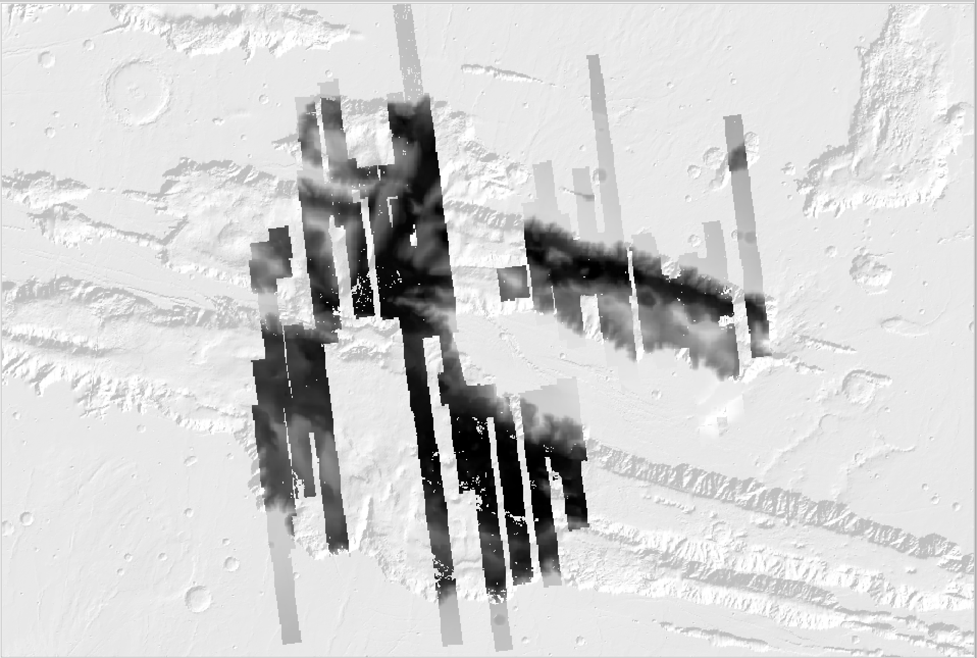
The MOLA shaded relief, or hillshade product provides the background context for this figure. A GDAL VRT containing 83 DTMs is overlayed to illustrate the differences between a DTM, where height is represented by intensity and a hillshade, where height is accentuated by shading caused by an artificially placed light source.
To load the VRT into QGIS:
- In the menu bar open the Layer menu and choose Add Raster Layer
- In the Add Raster Layer window navigate to the directory where the VRT was created and select it.
- Click the Add button to add the VRT to the project.
Alternatively, simply drag the VRT from the directory it is saved in into the Table of Contents (lower left side of the QGIS window).
A GIF demonstrating loading a VRT into QGIS using the steps enumerated above.
The VRT that was created in the ROI contains 83 DTMs, but only a single layer is added to QGIS. Why is this? The VRT is a virtual mosaic of all of the DTMs and is effectively combined into a single raster layer. Therefore, it is important to note that this product does contain less data than one would have if they loaded in 83 individual DTMs. This produce also inevitably has small discontinuities in the $z$ dimension due to misalignments to MOLA1.
By adding the VRT first, the project SRS is set properly. If you have worked through our QGIS WMS tutorial , add the MOLA shaded relief product. If you haven’t, skip this step.
As indicated above, the order that data are loaded can matter. If the VRT is loaded first, the project’s spatial reference system will beIAU:2015_49910which is equirectangular Mars with a spherical body, ocentric latitude and a central longitude of 0. If the WMS layer is added first, the project’s CRS will remainEPSG:4326which is an Earth based system. If the MOLA shaded relief is added first, make sure to change the CRS toIAU:2015_49910.
To create the hillshade:
- Right click on the DTM in the Table of Contents (ToC) and select Properties.
- In the properties dialog, select Symbology.
- In the Render type dropdown, select Hillshade.
- Optional: Check the Multidirectional box (it makes a more even hillshade with less stark shadows).
- Change the Resampling (Zoomed In and Zoomed Out) to Bilinear or Cubic
- Set the Oversampling (in the Resampling area of the dialog) to 1.0.
A GIF demonstrating creating a pretty hillshade using the DTM VRT.
If you are interested in all of the other options in the dialog, make sure to checkout this terrific tutorial .
The hillshade created above is in grayscale. If you like the look, skip this step. If you like the look of a colorized hillshade, this step is for you. To create the colorized layer:
- Add the DEM again to QGIS (using the same steps as step 3a) and make sure it is the top layer or right-click on the layer in the T0C and select Duplicate Layer.
- Right click on the DTM in the ToC and select Properties.
- In the properties dialog select Symbology.
- In the Render type dropdown select Singleband pseudocolor (this is the first step that is different than the steps taken to make the hillshade).
- Choose a color ramp that you like (maybe making sure it is colorblind safe? ) and click Apply (to preview) or Ok (to close the dialog box).
A GIF demonstrating creating a single band colorized layer using a VRT DTM.
The colorized layer is overlayed with and obscuring pretty the hillshade. To fix this and visually combine the layers:
- Reopen the Symology dialog (steps 2 & 3 above).
- In the Blending mode dropdown select Multiply.
Now you should see a colorized layer and the pretty hillshade underneath. These are still two layers in QGIS, but are rendering as a colorized hillshade in the main map area.
A GIF demonstrating blending the single band colorized layer with the hillshade.
Finally, lets create an interactive 3D map view of the colorized hillshade. This section draws heavily from the terrific tutorial by Stephanie available here . To create the visualization:
- Open the View menu in the top menu bar and select New 3D Map View
- In the newly opened dialog, click Configure (under the wrench icon).
- For the Elevation layer select the hillshade created above.
- Set the Vertical scale to 2.5 (to get a nice z exaggeration in the heights).
- Set the Tile resolution to 1024px. The GIF demonstrates the default 16px, 512px, and 1024px. This setting effects the resolution of the visualization.
A GIF demonstrating blending the single band colorized layer with the hillshade.
You should now see a 3D visualization of the 83 DTM VRT, streaming off of an offsite S3 bucket. You can pan/zoom this visualization (hold shift to switch between panning and rotating.) You can also grap the whole Map View 1 window and embed it next to (or above/below) the initial 2D visualization. This way, you can see both the top down view and the 3D DTM at the same time.
That’s it! You now have a 3D, colorized hillshade to play around with. You also know how to search for DTMs from our API , create a VRT from results, load the VRT into QGIS, and create a very cool looking colorized hillshade. Fun next steps might be to try and render a flyover or add the MOLA shaded relief into the 3D visualization as a background layer.
If you have questions, comments, or a visualization to share, consider chatting below.
Any use of trade, firm, or product names is for descriptive purposes only and does not imply endorsement by the U.S. Government.
-
How is it possible that overlapping DTMs are not in perfect alignment? During product generation, each DTM is aligned to MOLA and then groups of DTMs are further aligned. These multiple alignment steps result in very good accuracy to the MOLA point cloud. There are two primary sources of error in this process that result in small misalignments: (1) the MOLA point cloud is sparse and so alignment of a dense DTM point cloud to a sparse MOLA point cloud inevitably has error and (2) each MOLA spot is not an infinitesimally small physical point on the ground, but a large circular polygon. The larger that spot on the surface the more the DTM point can ‘bounce’ around inside the MOLA spot. ↩︎