

Querying for data in an ROI and loading it into QGIS
This is an in progress draft example. Please feel free to test, but use with caution!
In this example, we are going to prepare data in order to visualize observations in the area around the Apollo 15 landing site. At the time of writing, we have only made available the monoscopic KaguyaTC data and this example returns ten images in our region of interest. In the future many more visible observations (as well as other data types such as DTMs) will likely be returned.
At the end of this example, you should have a handful of data products local to your computer and a QGIS project with those observations loaded over a WMS base map (for context). More importantly, this example should be a pretty solid cookbook that you can modify and use for other areas on the moon or other bodies.
Notes are included in this example to highlight areas that are ideal for a user to begin altering for their own use case.
This example builds off the command line interface tutorial and assumes that the reader already has a working stac-client conda environment with pystac-client and jq installed. If not, check out that tutorial first.
The region of interest that we want to explore is around the Apollo 15 landing site. We build a GeoJSON ROI and save that to a file. In this case, we call is roi.geojson.
{
    "type": "Polygon",
    "coordinates": [
      [ [3.1, 25.6 ], [4.1, 25.6], [4.1, 26.6], [3.1, 26.6], [3.1, 25.6] ]
    ]
}
A user could define any ROI that they were interested in, by modifying the above bounding box, or passing in a more complex geometry.
Now execute the query to find data that intersects the area of interest and with a target of the moon.
stac-client search https://stac.astrogeology.usgs.gov/api/ --intersects aoi.geojson -q 'ssys:targets=moon' --save apollo15.geojson
Reminder, if you want to see how many observations this will return before downloading the GeoJSON response, replace --save <some name> with --matched.
Multiple different options for installing QGIS exist. One could download QGIS from the official download page or use conda to install QGIS via the command line .
At the time of writing, we would suggest using the official download source as the build is a little more ‘full featured’, but either installation method will work for this example.
For this example, two different options exist for setting the map projection. One option would be to use the already encoded Geographic Coordinate System (GCS) Moon 2000 projection. This is the spherical (units are latitude / longitude) as defined by the International Astronomical Union (IAU). The other option is to load one or more of the analysis ready observations and let QGIS default to the Universal Transverse Mercator (UTM) projection that the COGs are provided in. For now, we’ll use GCS_Moon_2000.
We are planning a number of learning pages on map projections and the tradeoffs inherent in the decision above.
To set the projection to GCS_Moon_2000, see the wonderful QGIS documentation on project projections .
You will know that the project projection is correctly set when the status bar at the bottom of QGIS shows the projection as ESRI:104903.

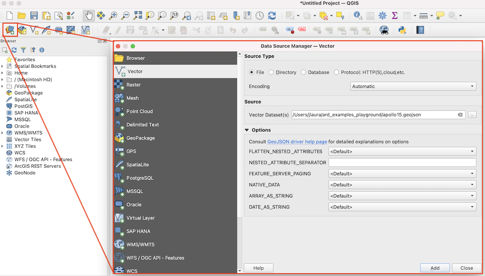
Now that the projection is properly set in QGIS, it is time to load the query response and get on with an analysis. To load a vector layer, click the Data Source Manager button in the top toolbar, select Vector, and navigate to the location where you saved the apollo15.geojson file.
The Data Source Manager should look similar to the screen capture below:
Once loaded (and stylized if you like ), you should see the footprints of the observations.
It is convenient to have a base map when performing an analysis in order to provide context for individual observations. Instead of downloading a, potentially quite large, base map, we instead stream the basemap from a remote server using the WMS specification. Luckily, QGIS makes it quite easy to add a WMS server and select an available base layer.
https://planetarymaps.usgs.gov/cgi-bin/mapserv?map=/maps/earth/moon_simp_cyl.map
Other WMS endpoints are provided by the USGS Astrogeology Science Center. For example:
- Mars: https://planetarymaps.usgs.gov/cgi-bin/mapserv?map=/maps/mars/mars_simp_cyl.map
-Europa: http://planetarymaps.usgs.gov/cgi-bin/mapserv?map=/maps/jupiter/europa_simp_cyl.map
In the browser on the left hand side of the QGIS application, select WMS->New Connection....
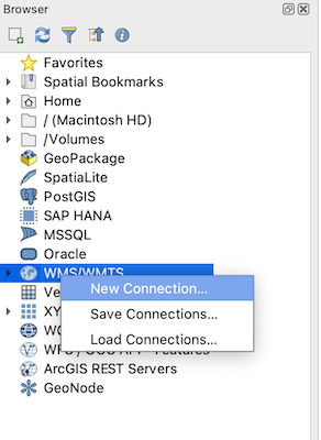
In the window that opens, name the connection and post the above Moon URL into the URL bar.
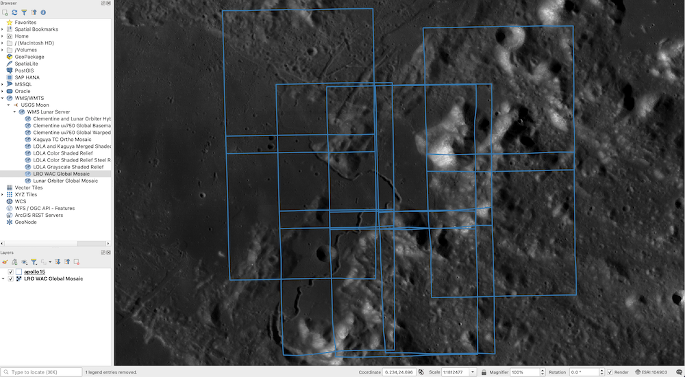
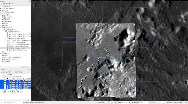
For this example, we select the LRO WAC Global Mosaic for context and double-click it to add it to the project. In the screen capture below, we have dragged the geojson layer above the WMS base in the list of layers so that the footprints are drawn on top of the basemap.
For this next step, bonce back over to the terminal where the query was executed. We want to get the data URLs (i.e., the observations) from the features in the GeoJSON response from our previous query. Just like in the
CLI tutorial
, the jq command line tool will be used.
First, let’s print the URLs to the screen as a sanity check: jq ‘.features[].assets[] | select(.key==“image”) | .href’ -r apollo15.geojson
The result should look like the following:
|
|
Assuming that that looks good, pipe the results to a file that will be used later:
jq ‘.features[].assets[] | select(.key==“image”) | .href’ -r apollo15.geojson > vrts2build.lis
Since we just printed a number of URLs for the observations to the screen, let’s go ahead and add one manually to QGIS. To do this, copy one of the URLs and then open the Data Source Manager (just like we did above to add the Vector GeoJSON data). This time, select Raster, set the Source Type to HTTP(S), Cloud, etc., and paste the copied URL into the box labelled URI. The window should look similar to this screen capture:
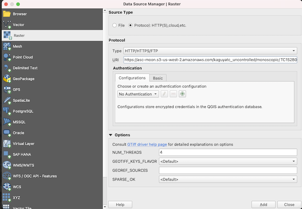
We have found that it is important to set the NUM_THREADS option to some number greater than 4 in order to get a performant load of the data. Once loaded, this option does not seem to impact rendering (panning and zooming is very fast), but the initial load can feel slow (not instantaneous as one would expect) without setting this option.
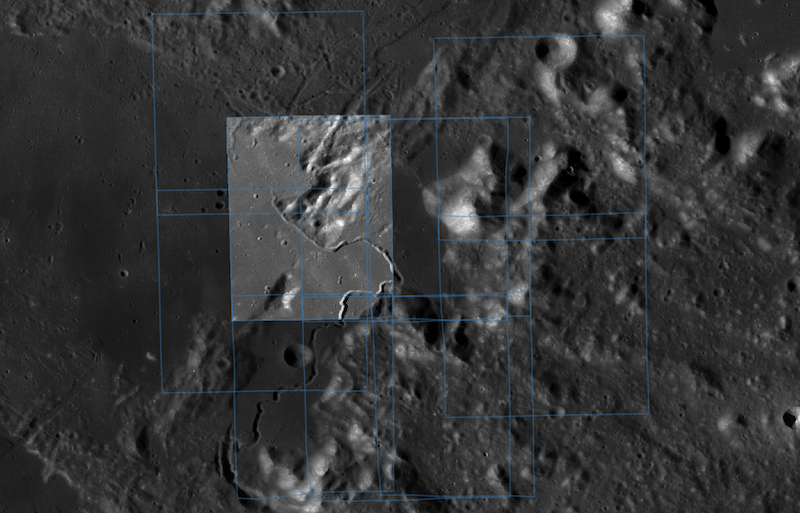
Once you click ‘Ok’, QGIS will load the COG. For example, we loaded: https://asc-moon.s3-us-west-2.amazonaws.com/kaguyatc_uncontrolled/monoscopic/TC1S2B0_01_05187N265E0029/TC1S2B0_01_05187N265E0029.tif to generate the screen capture below:
Imagine for a moment that a query is being run for hundreds if not thousands of observations in some region of interest. Adding each individually to QGIS would be prohibitive to say the least. Instead of loading each individually, we will make a VRT (described below) for each observation.
The GDAL Virtual Format or VRTs are tiny, XML text files that point to one or more images, subsets of images, remote resources, etc. We are using a VRT because QGIS allows one to load many on disk files at once (as opposed to one remote file at a time via the Data Source Manager). Hopefully in the future, we can remove this step.
Why many VRTs and not a single VRT? A single VRT can include many images. Those images are a virtual mosaic, where the ordering in the XML file defines which pixels are observed. If one wished to create a single mosaicked observation, it would make sense to build a single VRT. For this example, we want to see the individual observations, so we need one VRT for each COG.
Additionally, the KaguyaTC data are intentionally captured to accentuate topography. A great way to do that is with potentially extreme shadows. If one wished to build a mosaic, it would be important to use the query capabilities to further filter the data on view geometry (such as view:off_nadir>15). Without a filter, the dynamic ranges of the data sets (the DNs) is sufficiently divergent that visualization is problematic - see more below.
Back in the terminal, we will create one VRT for each observation in our query. A sample script that does this is copied below. Copy that script to a text file and name it urls2vrt.sh.
|
|
To run the script, simply execute:
urls2vrt.sh vrts2build.lis
After a few moments, you should see 10 VRTs on disk.
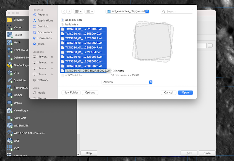
Finally, the VRTs are loaded by opening the Data Source Manager, selecting Raster, clicking the ellipses and selecting all ten VRTs.
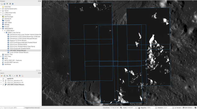
Warning! The results are pretty disappointing, but we will fix that.
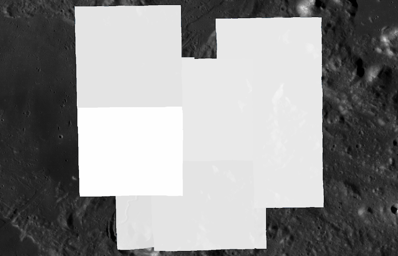
What we really need to do, is figure out which data have similar viewing geometries, and therefore similar illumination conditions. Then, the like image data can be grouped a similar stretches applied. A bit of exploration of the data, turning images on and off via the layer browser, and viewing the
image histograms
leads us to set the min/max for some of the observations to 0 - 20 and for others to -1 - 10. Looking at the
attribute table
, we see that the light images consistently have view:off_nadir angles greater than 15 and the dark images have view:off_nadir angles less than 15.
To get q bit more organized, we group the data based on observation geometry. The final results are shown below.
We did a bit of work to subset the data based on an attribute in the GeoJSON (view:off_nadir). Instead of doing this within QGIS, what would need to be added to the initial query to only get images with view:off_nadir>15?
In this example, you have queried the USGS STAC endpoint for lunar data in the area of the Apollo15 landing site. We have added that data to a QGIS project with the appropriate coordinate reference system (CRS). We have loaded vector (GeoJSON) data that is the response from the query and then parsed those results to stream observations into QGIS over a WMS basemap. Finally, after a bit of exploratory data analysis, we discovered that the view geometries are very divergent between observations and have subset the data into higher and lower incidence angles (off_nadir).