Mosaic.json Analysis
This is an in progress draft example. Please feel free to test, but use with caution!
In this tutorial we will demonstrate how to use the mosaic.json document created in the prior tutorial with Rasterio and QGIS for use in analysis.
Users will need a python environment with the following dependencies installed. The python environment made within the mosaic.json python tutorial has all of these dependencies included already except for matplotlib.
- rasterio
- httpx
- matplotlib
- uvicorn
- planetcantile
TiTiler is a light-weight python based dynamic tile web server that is open source and freely made available and maintained by the company DevelopmentSeed. TiTiler uses TileMatrixSets to efficiently provide REST endpoints to work with COGs and mosaic.json documents, enabling basic metadata queries and more advanced operations such as dynamic reprojection, resampling, rescaling, and advanced user made algorithms computed on a per-tile basis. TiTiler also helps traditional GIS analysis applications like QGIS make use of newer standards like mosaic.json.
For this tutorial we will use the TiTiler application included with Planetcantile for working with our mosaic.json documents both programmatically and with QGIS.
Users will also need access to a TiTiler endpoint that uses the Planetcantile TileMatrixSet definitions discussed in the mosaic.json tutorial. Users who have installed Planetcantile may use the TiTiler app included within Planetcantile, or they can connect to the one hosted by the USGS astrogeology center at <>.
To launch the Planetcantile TiTiler app, in another terminal run
|
|
Which will launch a webserver for TiTiler on you machine.
Let this process continue to run as you proceed through the terminal, but it can be shutdown whenever you are no longer using it.
Using TiTiler’s REST api, we will make some basic queries demonstrating use of our mosaic.json documents. First we will copy the mosaic.json files (assuming they are in the current working directory) to /tmp/ for shorter file paths later on in the tutorial.
|
|
Next we will perform some imports
|
|
And next we will define some paths we will re-use.
|
|
First we will use the mosaicjson/info endpoint provided by TiTiler to output basic information about the mosaics we’ve made.
|
|
Info for /tmp/jezero_ctx_hillshade_py_mosaic.json:
{ 'bounds': [ 75.91771659930976,
              14.65135146010114,
              77.90597708129924,
              19.777888275132497],
  'center': [76.91184684030449, 17.21461986761682, 0],
  'crs': 'http://www.opengis.net/def/crs/IAU/2015/49900',
  'mosaic_maxzoom': 25,
  'mosaic_minzoom': 9,
  'mosaic_tilematrixset': "<TileMatrixSet title='Mars (2015) - Sphere EN "
                          "MercatorSphere' id='MarsMercatorSphere' "
                          "crs='http://www.opengis.net/def/crs/EPSG/0/None>",
  'name': 'Jezero Example Hillshade',
  'quadkeys': []}


Info for /tmp/jezero_ctx_ortho_py_mosaic.json:
{ 'bounds': [ 75.91771659930976,
              14.65135146010114,
              77.90597708129924,
              19.777888275132497],
  'center': [76.91184684030449, 17.21461986761682, 0],
  'crs': 'http://www.opengis.net/def/crs/IAU/2015/49900',
  'mosaic_maxzoom': 25,
  'mosaic_minzoom': 9,
  'mosaic_tilematrixset': "<TileMatrixSet title='Mars (2015) - Sphere EN "
                          "MercatorSphere' id='MarsMercatorSphere' "
                          "crs='http://www.opengis.net/def/crs/EPSG/0/None>",
  'name': 'Jezero Example Orthos',
  'quadkeys': []}


Info for /tmp/jezero_ctx_dtm_py_mosaic.json:
{ 'bounds': [ 75.91771659930976,
              14.65135146010114,
              77.90597708129924,
              19.777888275132497],
  'center': [76.91184684030449, 17.21461986761682, 0],
  'crs': 'http://www.opengis.net/def/crs/IAU/2015/49900',
  'mosaic_maxzoom': 25,
  'mosaic_minzoom': 9,
  'mosaic_tilematrixset': "<TileMatrixSet title='Mars (2015) - Sphere EN "
                          "MercatorSphere' id='MarsMercatorSphere' "
                          "crs='http://www.opengis.net/def/crs/EPSG/0/None>",
  'name': 'Jezero Example DTMs',
  'quadkeys': []}
Next we can use the assets endpoint for mosaicjson that returns the actual COGs used for a given bounding box that is encoded as part of the url path. In the example below we requested the assets needed for the bounding box with a min longitude of 75 degrees, a max longitude of 76 degrees, a min latitude of 14 degrees, and a max latitude of 16 degrees. As the bounds of the mosaic are largely controlled by one very “long” CTX product, and we placed the bounding box in a corner of the extent where it should only intersect that asset.
|
|
Asset Info for /tmp/jezero_ctx_hillshade_py_mosaic.json:
[ 'https://astrogeo-ard.s3-us-west-2.amazonaws.com/mars/mro/ctx/controlled/usgs/P05_002809_1975_XI_17N283W__P13_006000_1974_XI_17N283W/P05_002809_1975_XI_17N283W__P13_006000_1974_XI_17N283W_hillshade.tif']
Next, we will use the point endpoint to ask for the assets that would be accessed for a particular coordinate. We will use a longitude and latitude in Jezero Crater near the Three Forks location and the front of the western fan.
|
|
Point Info for /tmp/jezero_ctx_dtm_py_mosaic.json:
{ 'coordinates': [77.41359752, 18.45369687],
  'values': [ [ 'https://astrogeo-ard.s3-us-west-2.amazonaws.com/mars/mro/ctx/controlled/usgs/P18_007925_1987_XN_18N282W__P19_008650_1987_XI_18N282W/P18_007925_1987_XN_18N282W__P19_008650_1987_XI_18N282W_dtm.tif',
                [-2515.744140625],
                ['b1']],
              [ 'https://astrogeo-ard.s3-us-west-2.amazonaws.com/mars/mro/ctx/controlled/usgs/P02_001820_1984_XI_18N282W__P06_003442_1987_XI_18N282W/P02_001820_1984_XI_18N282W__P06_003442_1987_XI_18N282W_dtm.tif',
                [-2495.833740234375],
                ['b1']],
              [ 'https://astrogeo-ard.s3-us-west-2.amazonaws.com/mars/mro/ctx/controlled/usgs/N03_063453_1982_XN_18N282W__N03_063519_1982_XN_18N282W/N03_063453_1982_XN_18N282W__N03_063519_1982_XN_18N282W_dtm.tif',
                [None],
                ['b1']],
              [ 'https://astrogeo-ard.s3-us-west-2.amazonaws.com/mars/mro/ctx/controlled/usgs/N01_062952_1988_XN_18N282W__N01_062662_1988_XN_18N282W/N01_062952_1988_XN_18N282W__N01_062662_1988_XN_18N282W_dtm.tif',
                [-2539.234375],
                ['b1']]]}
Getting to more practical applications, below we demonstrate various ways to use the mosaic.json documents with TiTiler in commonly used analysis software such as QGIS for direct use in a GIS environment like any other geospatial dataset users are familiar with, and Rasterio, a popular python wrapper for the GDAL API. In both cases it is possible to access the full floating point precision data offered by the DTM and Orthoimage ARD COGs in the mosaic without needing to connect to all of the COGs individually or using GDAL’s VRT format which doesn’t optimize for image overlaps like the mosaic.json format does.
To view the mosaic.json mosaics in QGIS we will need to use the WMS driver within GDAL, specifically the TMS minidriver to define xml files that point to the mosaic.json document we are interested in viewing and insert other metadata that is needed by hand. Unfortunately there is no automated option currently for generating these yet, but eventually we hope to provide such tools. In the end the XML file tells GDAL how to request tiles correctly from the TiTiler server.
More details about the GDAL WMS driver can be found
here
, but in brief
the most important parameter is the <ServerURL>...</ServerURL> information. There we need to use the mosaicjson/tiles TiTiler endpoint to request tiles for the mosaic.json document that we pass in via the url parameter. Be aware that running the TiTiler endpoint yourself could cause files to no longer work if the port number for TiTiler changes, but using the USGS TiTiler instance should avoid that issue. The section ${z}/${x}/${y}@1x.{format} critically defines the schema GDAL will use to make requests for tiles, and the file extension which will be critical for allow us to access floating point data provided by the DTM and Orthoimage mosaics, which will require the use of the .tif file extension, also used in the <ImageFormat> tag.
Next the <DataWindow> needs to be specified to match the information for the TileMatrixSet, which means defining the maximum bounds in the projection (in this case MarsEquidistantCylindricalSphere or IAU_2015:49910) and specifying the tile aspect ratio via the <TileCountX/Y> options which here say that our tile grid has twice as many tiles in the X axis as the Y axis. From the prior tutorial on mosaic.json, we used the MarsMercatorSphere TMS to define the mosaic.json file, however there is no requirement that similar mercator projects be used for viewing the mosaic.json document. Although we do not demonstrate it here, it is possible to use other projections and geographic CRSs with this mechanism.
Next we fill out some other important metadata like the tile size via the BlockSize parameters, which needs to match the tile size used in the TMS, the band count, and the data type.
Critically for our DTM and Ortho mosaic products, we will use the Float32 datatype so that we can get the data at full precision into our visualization in QGIS. However it is also possible to use TiTiler to rescale the data which we will demonstrate in a later section.
Once these files are created it is possible to simply drag and drop them into a QGIS project to view them. You may notice some initial delay required by the TiTiler server that could last 10s of seconds, but after the map will be usable at typical speeds. You may also have to adjust the styling for the layers if QGIS doesn’t respect the data range you specified in the xml files.
|
|
Overwriting jezero_mosaic_json_hillshade.xml
|
|
Overwriting jezero_mosaic_json_ortho.xml
|
|
Overwriting jezero_mosaic_json_dtm.xml
As loading these files is as simple as dragging and dropping the files into the QGIS interface, we will not demonstrate that, but instead we will display some screenshots of the application using the layers.
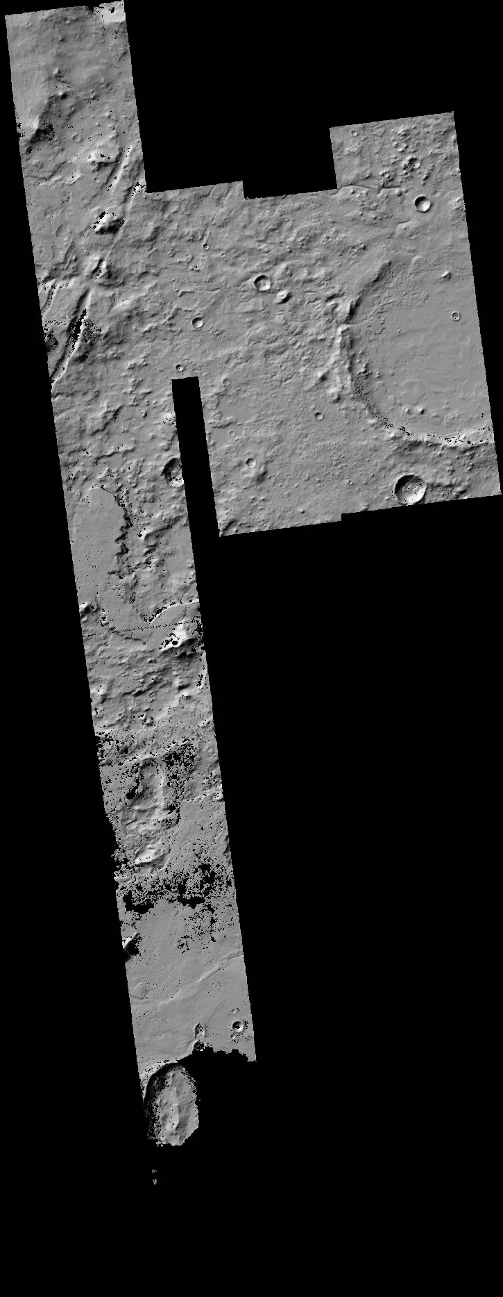
First let’s see the whole extent of the hillshade mosaic.
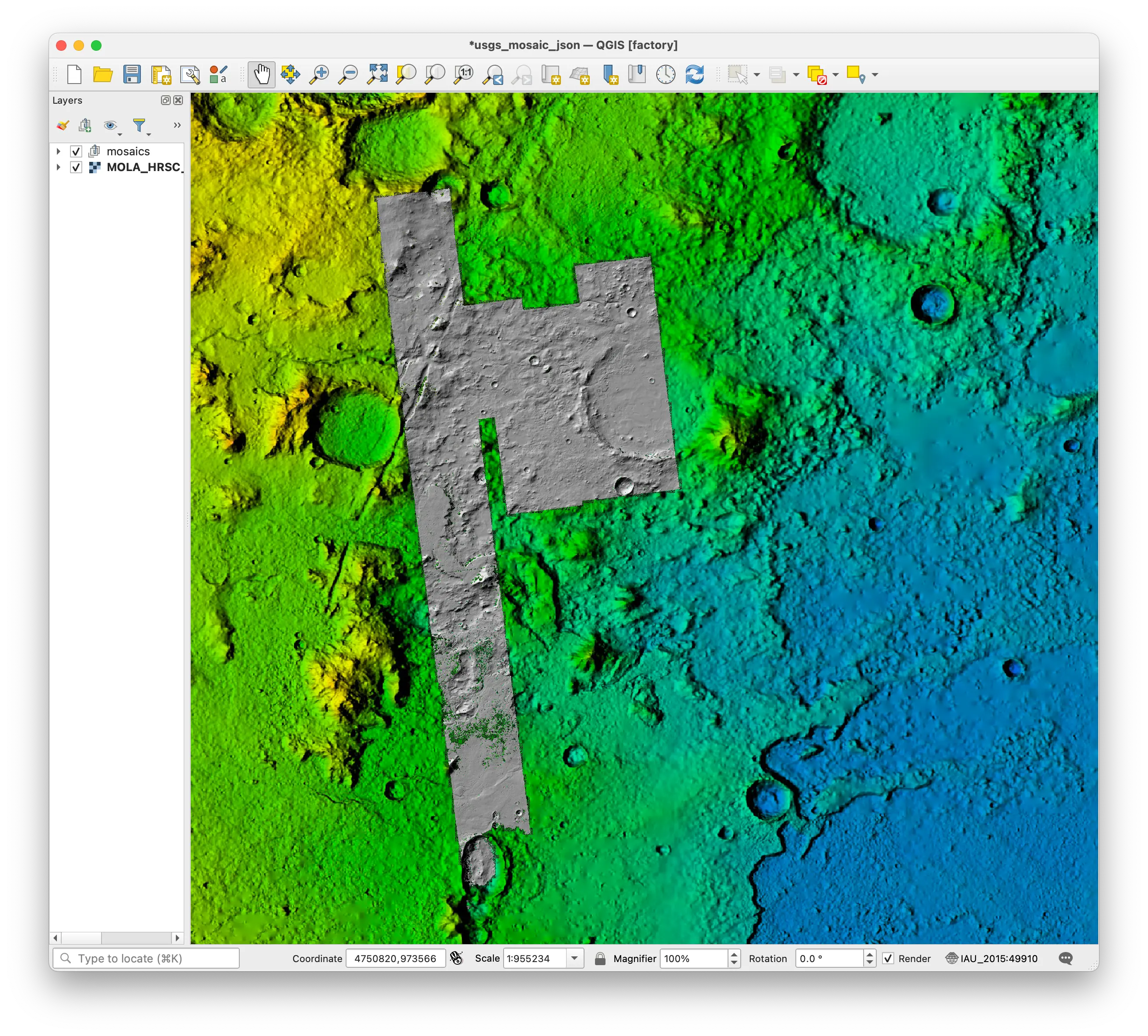
Zooming in we can see more detail at Jezero crater.
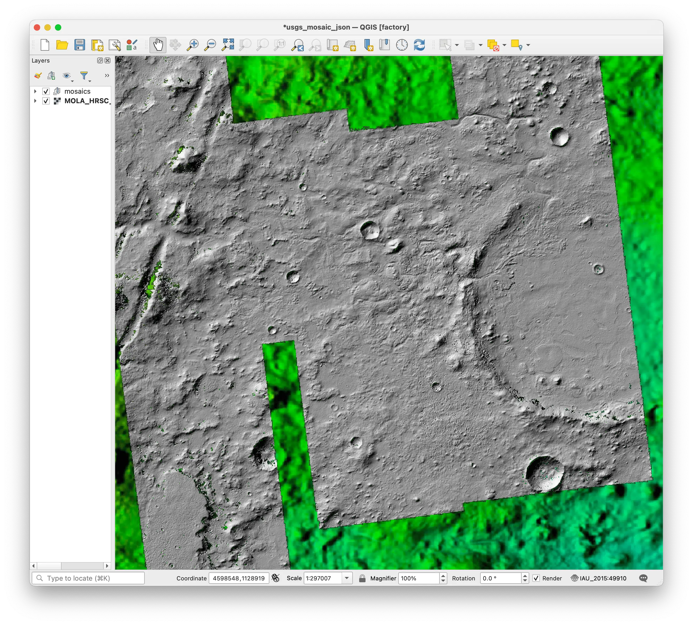
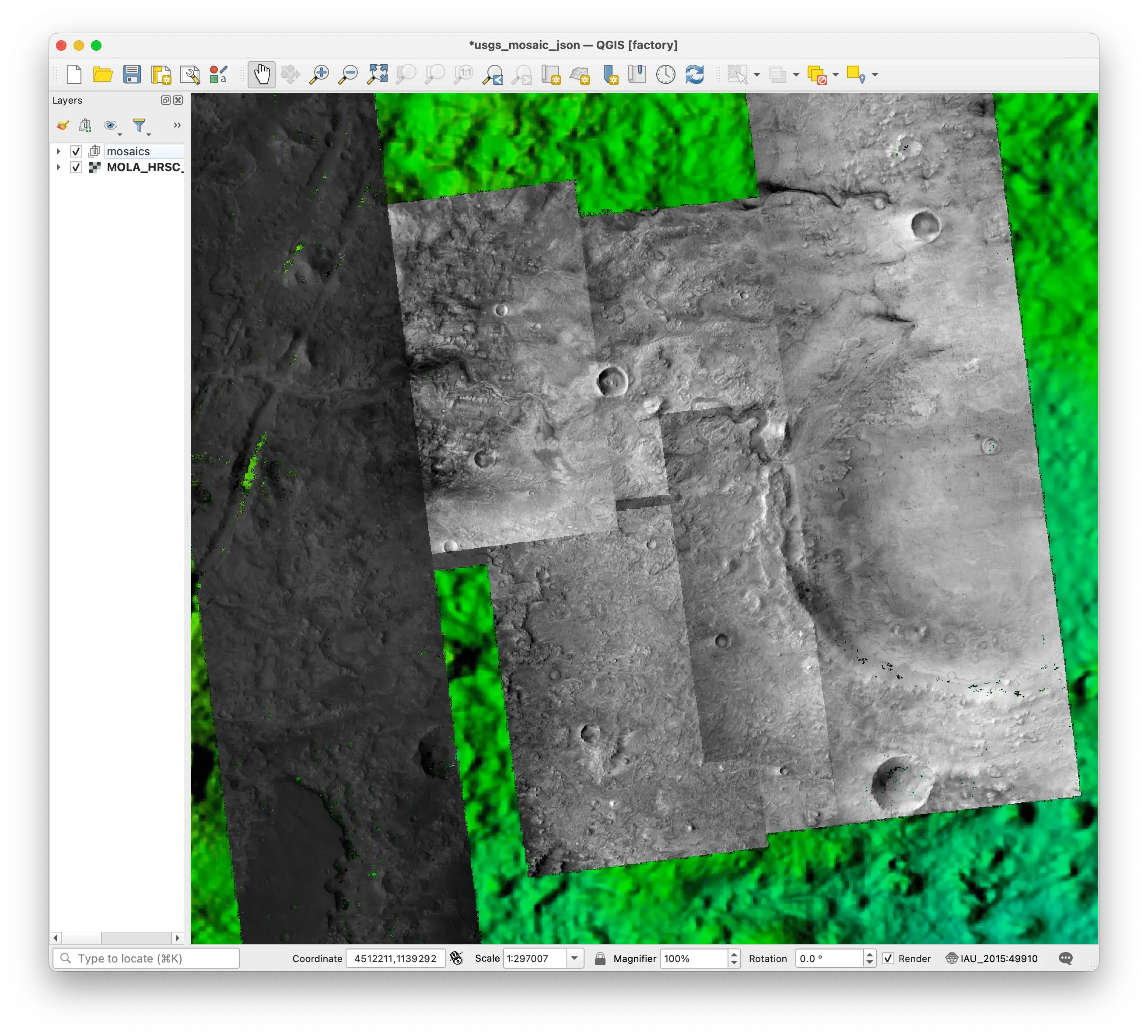
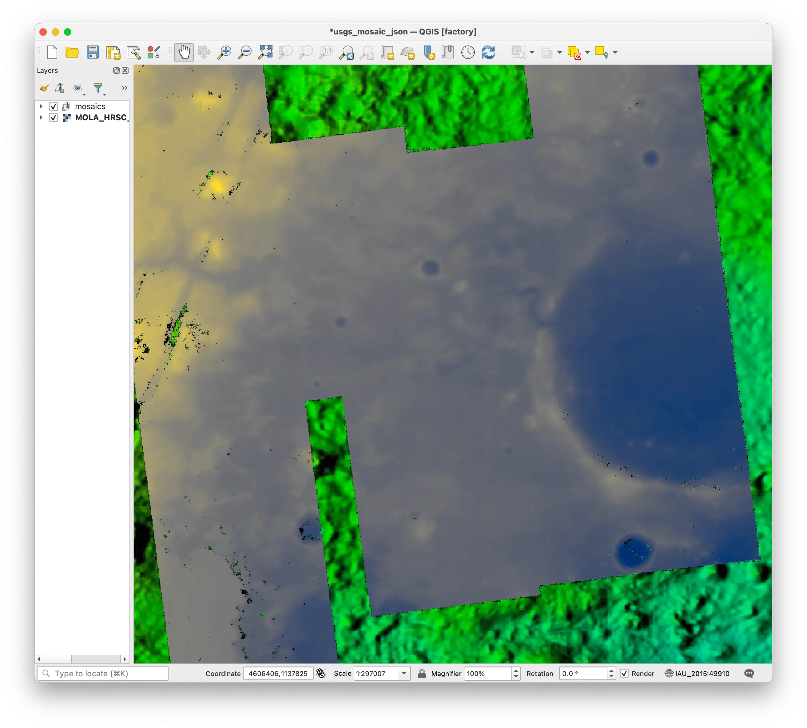
Next we can display the ortho image mosaic. Due to the processing of the ortho mosaic products, the brightness of the various images is not uniform resulting in sharp changes where assets overlap
The DTM mosaic can be styled using QGIS layer options like any raster dataset, so we used the cividis colormap and scaled the data to the elevation range of -3200m to 0m.
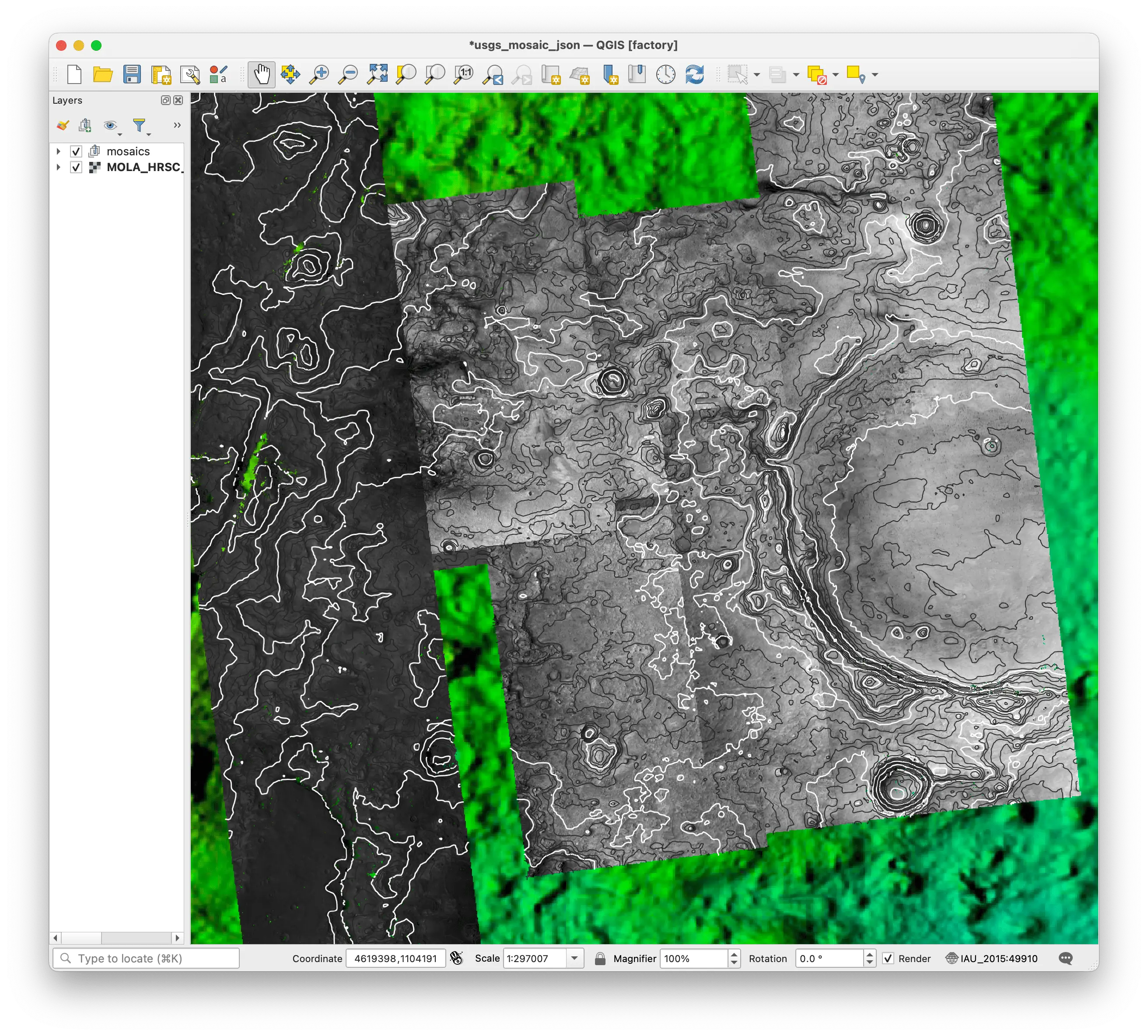
As QGIS provides powerful features such as on-the-fly contour computation, we can make a copy of the DTM map layer with the contour style applied and see it overlain ontop of the ortho mosaic. Contours are every 50 meters of elevation with index levels every 250 meters in white.
In addition to the WMS driver, the WMTS driver in GDAL better supports the TileMatrixSets and follows a very similar XML format to the WMS XML files we created above, however these files don’t seem to work in QGIS directly but will work in tools like Rasterio and the GDAL command line. Conversely, the WMS XML files don’t seem to work well with Rasterio which benefits from more precise extent information. More information about this driver is available here .
First we will use the WMTSCapabilities.xml endpoint from TiTiler to get the Capabilities xml documents for the mosaics. These contain metadata including the url GDAL and other tools will use to get tiles internally and the TileMatrixSet. As before we need to adjust the tile_format parameter if we wish to access the DTM and Ortho products at their native bit depth.
|
|
WMTS for /tmp/jezero_ctx_hillshade_py_mosaic.json written to /tmp/jezero_ctx_hillshade_py_mosaic_wmst.xml


WMTS for /tmp/jezero_ctx_ortho_py_mosaic.json written to /tmp/jezero_ctx_ortho_py_mosaic_wmst.xml


WMTS for /tmp/jezero_ctx_dtm_py_mosaic.json written to /tmp/jezero_ctx_dtm_py_mosaic_wmst.xml
Although GDAL can partially use these files alone, we need to do additional work similar to the WMS XML we created earlier. First we will need the precise bounds for the mosaics using the bounds endpoint in TiTiler.
|
|
Bounds for /tmp/jezero_ctx_hillshade_py_mosaic.json:
{ 'bounds': [ 4499999.688084169,
              868454.426105146,
              4617853.226751639,
              1172328.3451582233],
  'crs': 'http://www.opengis.net/def/crs/IAU/2015/49910'}


Bounds for /tmp/jezero_ctx_ortho_py_mosaic.json:
{ 'bounds': [ 4499999.688084169,
              868454.426105146,
              4617853.226751639,
              1172328.3451582233],
  'crs': 'http://www.opengis.net/def/crs/IAU/2015/49910'}


Bounds for /tmp/jezero_ctx_dtm_py_mosaic.json:
{ 'bounds': [ 4499999.688084169,
              868454.426105146,
              4617853.226751639,
              1172328.3451582233],
  'crs': 'http://www.opengis.net/def/crs/IAU/2015/49910'}
Now that we know the bounds for the mosaics (of course they would all be the same), we can use these bounds within the <DataWindow> block of the <GDAL_WMTS> xml object. Below we will create all three files as we’ve done before, adjusting some parameters as needed for the floating point data.
|
|
Overwriting jezero_ctx_hillshade_mosaic_wmts.xml
|
|
Overwriting jezero_ctx_ortho_mosaic_wmts.xml
|
|
Overwriting jezero_ctx_dtm_mosaic_wmts.xml
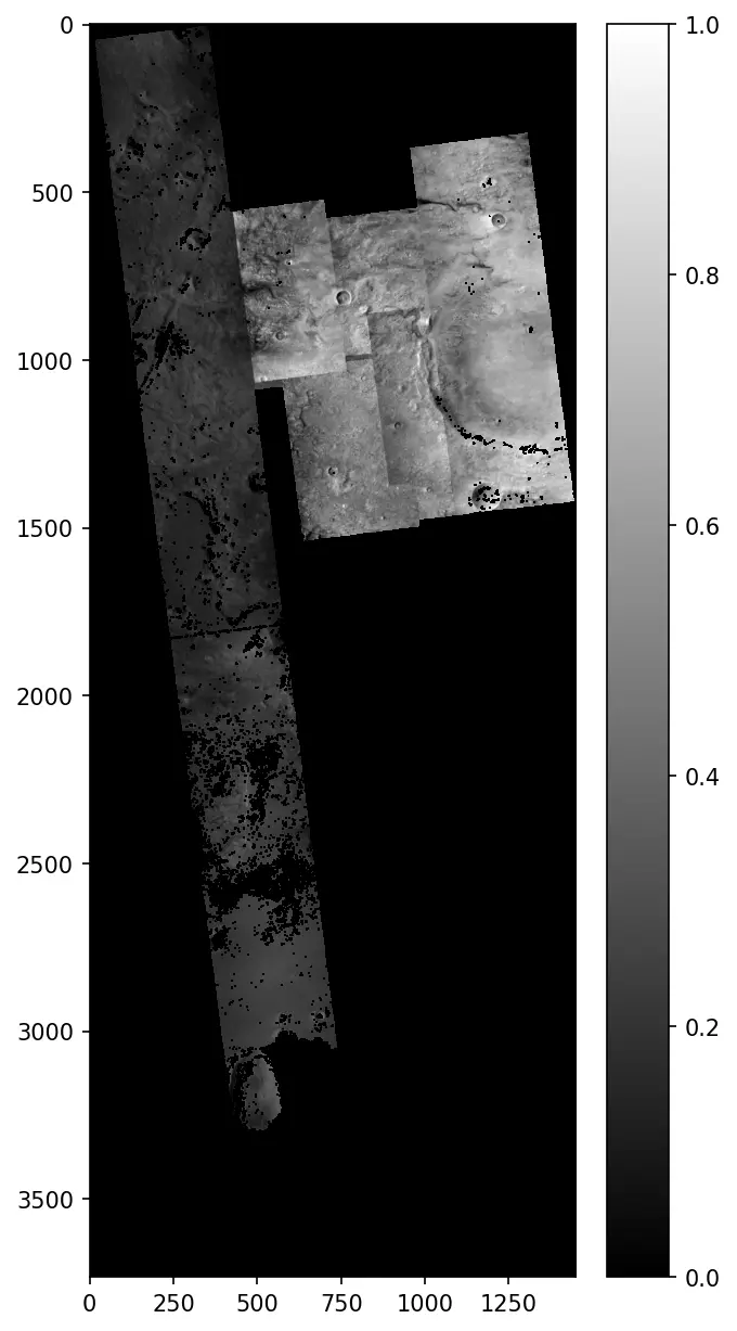
Now that we have the three _wmts.xml files we can begin to use rasterio to access the data from the mosaics in Python. We will use the rasterio.open function (rio.open) to open the xml file like any other raster file. The only additional parameter to pay attention to is the zoomlevel which is critical for mosaics where if the data was extracted at their native resolution would result in far too many tiles requested of the server for simple previewing. We will set this parameter to 8 and demonstrate what happens when a larger zoom level (more zoomed) query is performed.
Rasterio will return a numpy array that we can display inline with Pillow.
|
|
725 1867
For floating point data like the ortho mosaics we will need to use matplotlib to display the data in grayscale.
|
|
725 1867

Next we will do the same request except we will ask for zoom level 9, which will result in four times the number of pixels, and so will take longer to finish loading.
|
|
1448 3733
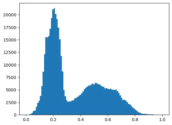
For more proof that the actual floating point data was loaded we can plot a histogram to demonstrate that:
|
|
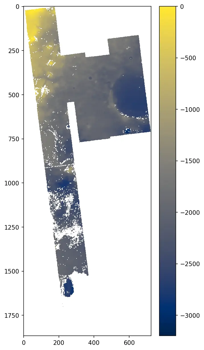
Next we will load the DTM mosaic with rasterio and display it with matplotlib. Due to some quirks with the GDAL WMTS driver and how empty tiles are handled, we will need to manually map values of 0.0 to the nodata value used of -32767.0 for the DTM products. We also then reassign those values to nan to permit better plotting in matplotlib. We will also plot the DTM with the cividis colormap to illustrate the elevation range in the data.
|
|
725 1867